The Main Principles Of Google Sheets Vlookup

Usage VLOOKUP when you require to find things in a table or a variety by row. For instance, look up a cost of an automotive component by the part number, or locate a worker name based upon their staff member ID. In its most basic type, the VLOOKUP function claims: =VLOOKUP(What you intend to seek out, where you wish to try to find it, the column number in the variety having the value to return, return an Approximate or Precise match-- indicated as 1/TRUE, or 0/FALSE).

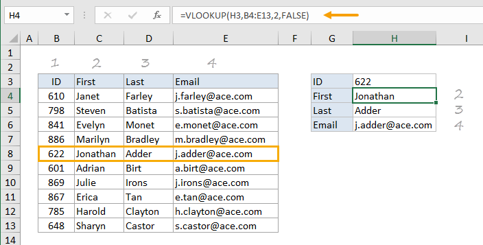
Use the VLOOKUP function to search for a worth in a table. Phrase structure VLOOKUP (lookup_value, table_array, col_index_num, [range_lookup] As an example: =VLOOKUP(A 2, A 10: C 20,2, REAL) =VLOOKUP("Fontana", B 2: E 7,2, FALSE) =VLOOKUP(A 2,'Customer Information'! A: F,3, FALSE) Debate name Summary lookup_value (needed) The worth you want to search for. The worth you wish to seek out must be in the first column of the series of cells you specify in the table_array debate.

Lookup_value can be a worth or a referral to a cell. table_array (required) The series of cells in which the VLOOKUP will certainly look for the lookup_value and the return value. You can use a named range or a table, and also you can use names in the argument rather of cell references.

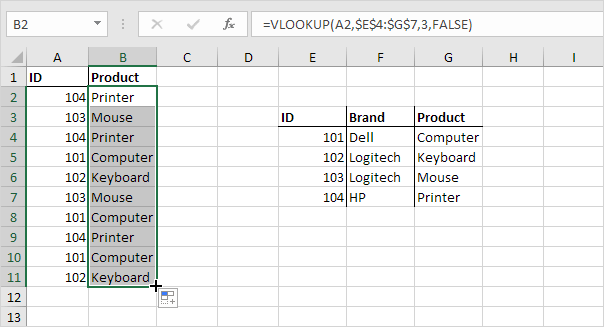
The cell range likewise needs to consist of the return value you wish to locate. Find out just how to pick varieties in a worksheet. col_index_num (called for) The column number (starting with 1 for the left-most column of table_array) which contains the return worth. range_lookup (optional) A logical worth that defines whether you want VLOOKUP to find an approximate or an exact match: Approximate match - 1/TRUE thinks the very first column in the table is arranged either numerically or alphabetically, and will certainly then look for the closest value.

For instance, =VLOOKUP(90, A 1: B 100,2, REAL). Exact suit - 0/FALSE searches for the exact worth in the very first column. As an example, =VLOOKUP("Smith", A 1: B 100,2, FALSE). There are 4 items of information that you will certainly need in order to develop the VLOOKUP syntax: The worth you intend to search for, additionally called the lookup worth.

Fascination About Excel Vlookup

Bear in mind that the lookup worth should constantly be in the initial column in the range for VLOOKUP to work appropriately. For example, if your lookup value remains in cell C 2 then your variety ought to start with C. The column number in the range which contains the return worth. As an example, if you define B 2:D 11 as the variety, you ought to count B as the initial column, C as the 2nd, and so forth.

If you don't specify anything, the default value will certainly constantly be TRUE or approximate match. Currently put all of the above with each other as complies with: =VLOOKUP(lookup value, array containing the lookup value, the column number in the variety including the return value, Approximate suit (TRUE) or Specific suit (FALSE)). Here are a few examples of VLOOKUP: Issue What failed Wrong worth returned If range_lookup holds true or omitted, the first column needs to be arranged alphabetically or numerically.

Either sort the initial column, or make use of FALSE for a specific match. #N/ A in cell If range_lookup is REAL, then if the value in the lookup_value is smaller than the smallest value in the very first column of the table_array, you'll obtain the #N/ A mistake worth. If range_lookup is FALSE, the #N/ A mistake worth suggests that the specific number isn't found.

#REF! in cell If col_index_num is higher than the variety of columns in table-array, you'll obtain the #REF! error value. To find out more on solving #REF! errors in VLOOKUP, see Just how to correct a #REF! mistake. #VALUE! in cell If the table_array is less than 1, you'll get the #VALUE! mistake worth.

#NAME? in cell The #NAME? error worth typically suggests that the formula is missing quotes. To seek out an individual's name, ensure you utilize quotes around the name in the formula. As an example, enter the name as "Fontana" in =VLOOKUP("Fontana", B 2: E 7,2, FALSE). For more details, see How to remedy a #NAME! mistake.

How Vlookup Example can Save You Time, Stress, and Money.

Learn how to use outright cell referrals. Don't keep number or day values as message. When looking number or day worths, make sure the data in the initial column of table_array isn't saved as text values. Or else, VLOOKUP might return an inaccurate or unexpected worth. Arrange the first column Type the very first column of the table_array before making use of VLOOKUP when range_lookup holds true.

An inquiry mark matches any solitary personality. An asterisk matches any type of sequence of personalities. If you wish to discover a real question mark or asterisk, kind a tilde (~) in front of the character. For instance, =VLOOKUP("Fontan?", B 2: E 7,2, FALSE) will certainly look for all circumstances of Fontana with a last letter that could vary.

When looking text values in the first column, see to it the information in the first column does not have leading spaces, trailing rooms, inconsistent use straight (' or") and also curly (' or ") quote marks, or nonprinting characters. In these instances, VLOOKUP might return an unanticipated worth.

You can always ask a specialist in the Excel Individual Voice. Quick Reference Card: VLOOKUP refresher course Quick Recommendation Card: VLOOKUP fixing tips You Tube: VLOOKUP videos from Excel area specialists Every little thing you require to understand about VLOOKUP Exactly how to fix a #VALUE! mistake in the VLOOKUP function Exactly how to correct a #N/ An error in the VLOOKUP feature Introduction of formulas in Excel Just how to stay clear of damaged solutions Identify errors in formulas Excel features (indexed) Excel features (by category) VLOOKUP (free sneak peek).

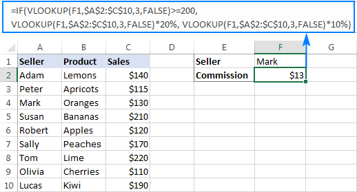
To compute delivery price based upon weight, you can use the VLOOKUP feature. In the instance shown, the formula in F 8 is: =VLOOKUP(F 7, B 6: C 10,2,1)* F 7 This formula uses the weight to locate the right "cost per kg" after that ... To override outcome from VLOOKUP, you can nest VLOOKUP in the IF feature.

excel vlookup query table excel vlookup in one column vlookup in excel column